
Modern portfolio theory is the most taught idea in investing and one of the most misunderstood. It won a Nobel Prize, it gave the world the phrase “diversification is the only free lunch,” and it genuinely changed how serious people think about risk. But somewhere between the 1952 paper and the sleek optimization dashboards sold today, a durable idea got dressed up as a machine that promises something it cannot deliver: the single mathematically optimal portfolio, computed from numbers you would have to know in advance. This guide separates the part of the theory worth keeping from the false precision layered on top — starting with the uncomfortable finding that the elaborate optimizer often loses to simply dividing your money evenly.
One Good Idea, Oversold
The insight at the core is real and was radical when Harry Markowitz set it out in his 1952 paper “Portfolio Selection,” arguing that an investor should not simply maximize expected return but weigh it against variance, and that a stock’s risk cannot be judged in isolation. What matters is how it moves in relation to everything else you hold. Two assets that each swing wildly but rarely swing together can combine into a portfolio steadier than either one alone — that is the “free lunch,” and it is why owning uncorrelated things beats owning more of the same thing. Markowitz shared the 1990 Nobel for this, and the idea deserves it. The blunt, everyday expression of it is the classic split between stocks and bonds, the logic behind the traditional 60/40 portfolio. The trouble begins only when “portfolio selection” gets sold as “portfolio optimization” — the promise of a precise best answer.
The Inputs Are Guesses
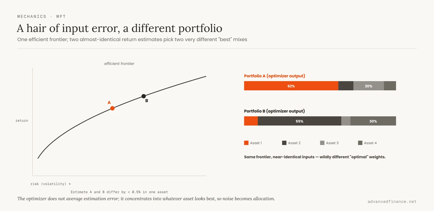
To compute the famous efficient frontier — the curve of portfolios offering the most return for each level of risk, with the “tangency” point that maximizes risk-adjusted return — the model solves a tidy piece of mathematics: choose the portfolio weights that give the smallest variance for a chosen level of expected return, or the most return for a chosen level of variance. The catch is what that calculation takes as fixed inputs. For every asset it needs an expected future return, and for every pair of assets it needs a variance and a covariance — an entire matrix of numbers describing how they will move together. Every one of those is unknown. In practice they are estimated from past data, and the past is a short, noisy sample of a system that keeps changing. Expected return is the worst offender: no honest analyst can tell you what stocks will return next decade to the decimal, yet the optimizer demands exactly that number. And it does not treat the errors gently. Hand it inputs that are slightly too optimistic on one asset and the optimizer piles into that asset, because its whole job is to chase the highest apparent reward-to-risk. It is, in effect, an error-maximizer wearing the costume of precision.
| Input the model needs | Where it comes from | Why it misleads |
|---|---|---|
| Expected returns | Extrapolated from history | Nearly impossible to forecast; tiny errors swing the “optimal” weights wildly |
| Volatilities | Measured from past prices | Calm periods understate it; volatility clusters and jumps in crises |
| Correlations | Measured from past prices | Not stable — they rise in downturns, exactly when you need them low |
Optimized vs Just Equal
If the input problem sounds academic, its consequence is brutally practical, and it has been measured. DeMiguel, Garlappi and Uppal tested fourteen versions of “optimal” mean-variance optimization across seven real datasets and found that none of them reliably beat the naive 1/N rule — simply splitting your money equally across the available assets — once they were measured out of sample on realistic data. The reason is exactly the one above: the theoretical gain from optimizing is more than offset by the estimation error in the inputs. Their sobering estimate is that you would need roughly 3,000 months of data — about 250 years — for a 25-asset optimizer to dependably outperform equal weighting. The lesson is not that diversification fails. It is that dividing sensibly beats optimizing precisely, because the precision is built on guesses. When a strategy this simple is this hard to beat, elaborate optimization is usually selling confidence, not returns.
The patches the pros use — and their limits
The profession knows all this and has built tools to blunt it, which are worth recognizing. Covariance shrinkage — the Ledoit-Wolf method is the best known — pulls the wild, noisy correlation estimates toward a stable average so the optimizer has less error to chase. The Black-Litterman model starts from the allocation the whole market is already holding and lets you nudge it only where you hold a genuine view, which stops the optimizer from betting everything on a single overstated return. Risk parity sidesteps expected-return forecasts almost entirely, weighting assets so each contributes the same amount of risk rather than the same number of dollars. Each of these is a real improvement. But notice what none of them do: escape the underlying problem. They make the estimates less fragile; they do not make the future knowable. A shrunk covariance matrix is still measured from the past, and a market-implied return is still a guess wearing humility. The patches lower the fever. They do not cure the illness.
When Diversification Fails
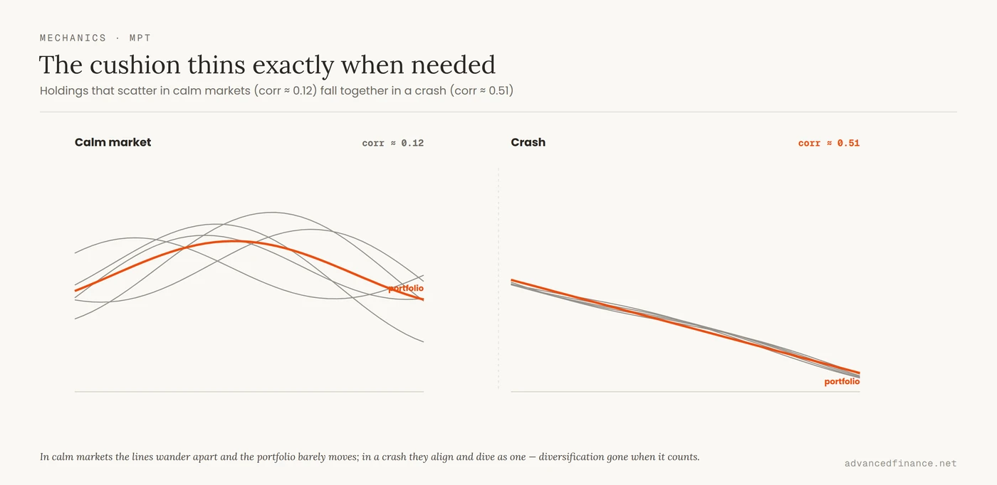
There is a deeper crack, and it opens at the worst moment. The correlations the model relies on are not just unstable — they move against you. Longin and Solnik showed that correlation between markets rises in bear markets but not in bull markets: in their data, extreme downward moves were correlated at around 0.51 across markets, while extreme upward moves correlated at only about 0.12. In plain terms, the assets that look pleasingly independent in a calm year tend to fall together in a crash. That is precisely what happened in 2008 and again in March 2020, when almost everything — including the “digital gold” that was supposed to be uncorrelated — sold off at once and the “diversified” portfolio offered far less shelter than its historical numbers promised. Diversification does not vanish, but the free lunch shrinks exactly when the bill arrives, which is why a basket of holdings that all ride the same engine — a dozen growth-tech names, say — is a single bet in disguise, and why reading fragility before a downturn matters more than any backtested correlation matrix.
| Market condition | Correlation of extreme moves | What it means for you |
|---|---|---|
| Extreme up-moves (bull) | ≈ 0.12 | Markets rise fairly independently — diversification looks great |
| Extreme down-moves (bear) | ≈ 0.51 | Markets fall together — the protection thins when you need it |
What Sharpe Actually Measures
Since every optimizer is chasing “the highest Sharpe ratio,” it is worth knowing what that number is and what it hides. In William Sharpe’s own description, the ratio is the expected return above the risk-free rate divided by the standard deviation of that excess return — in shorthand, (return − risk-free) ÷ volatility, or reward per unit of variability. It is a genuinely useful common yardstick, and Sharpe shared that same 1990 Nobel. But it carries two assumptions worth saying out loud. First, it is backward-looking: computed from history, it tells you what happened, not what will. Second, and more dangerous, it treats volatility itself as risk — punishing a big upside month exactly as much as a big downside one, and saying nothing about tail risk, drawdown, or the liquidity crunch that actually ends portfolios. That flaw has a known answer: downside-focused measures like the Sortino ratio, and the broader post-modern portfolio theory, replace total volatility with downside deviation so that only the variability that actually hurts counts against you. They are a real improvement on this one point — though they still lean on the same historical estimates as everything else here. Optimize blindly for a single backward-looking number and you end up precisely tuned for the last war: a strategy can post a beautiful Sharpe for years by quietly selling insurance against a crash that has not happened yet.
How To Actually Use It
None of this means throwing the theory out — it means using it as a way of thinking rather than a machine that hands you an answer. In practice that comes down to a handful of habits:
- Diversify by difference, not by count. Ten funds that all ride the same growth-tech engine are one position wearing ten names; the first honest task is to find where you are secretly concentrated across shared drivers.
- Prefer simple, robust weights. Equal or fixed rules-based weighting is brutally hard to beat, so treat an optimizer’s four-decimal output as a hypothesis to sanity-check, not an instruction to follow.
- Hold genuinely different return drivers. Broad regions, real assets, and documented factor tilts like value or quality — while remembering their independence is a calm-market feature that thins in a crash — because correlation is a regime that shifts with the macro shock, not a fixed property.
- Rebalance by threshold, not the calendar. Act only when an allocation drifts past a set band, so you harvest the premium without bleeding it away in taxes and trading costs.
- Keep a real liquidity bucket. Enough cash or high-quality bonds that a downturn never forces you to sell your worst-hit assets at the bottom — an easier discipline now that a higher-for-longer world actually pays you to hold cash.
- Choose an allocation whose ugliest year you could sit through. The plan you abandon in a panic was never optimal for you — which is a large part of why most long-term investors underperform their own funds.
FAQ
Is diversification still worth it if correlations rise in a crash?
Yes. It still lowers your everyday volatility and softens most ordinary drawdowns, which is most of what you experience as an investor. What it cannot do is protect you in a full systemic panic, when nearly everything falls together. For that, the only real defense is holding less risk overall — more cash or high-quality bonds — not a cleverer correlation matrix.
Should I use a portfolio optimizer?
Cautiously, and never on faith. The research is clear that optimizers rarely beat simple equal or rules-based weighting out of sample, because they amplify the estimation error in their inputs. Techniques like covariance shrinkage, Black-Litterman, and risk parity make them less fragile, but even those still rest on historical estimates. Use one to understand trade-offs, not to trust a set of weights calculated to four decimal places.
Is the 60/40 portfolio dead?
No, though 2022 gave that headline a lot of fuel, when stocks and bonds fell together during a sharp rate shock. That is a real weakness — bonds only cushion equities when they are not both being repriced by the same rising rates. But in most equity drawdowns the bond ballast still works, and “dead” overstates a blunt tool that keeps doing its blunt job.
What is the Sharpe ratio, exactly?
It is your return above the risk-free rate divided by the standard deviation of that excess return — reward per unit of volatility. It is a handy way to compare risk-adjusted performance, but it is backward-looking and treats all volatility as risk, so it can flatter a strategy that is quietly exposed to a rare, catastrophic loss. Downside-only measures like the Sortino ratio address that specific blind spot.
Can I use this theory with a small account under $10k?
Yes, and small is where it is easiest to do well, because simplicity is the winning move anyway. A handful of broad, low-cost, low-overlap funds, weighted roughly equally and rebalanced when they drift past a threshold, captures nearly all the real benefit of the theory and beats any optimizer at that size.
Author’s Insight
The mathematics seduced me early, the way it seduces most people who find it — there is something deeply satisfying about a curve that claims to show the single best portfolio. What cured me was watching those confident, four-decimal weights be the first thing to break whenever the market did something the history had not. The portfolios that actually survived were never the most mathematically optimal ones. They were the boring, roughly balanced ones I could hold through a bad year without flinching, because the entire value of a plan is whether you keep following it when it is losing. I still use the theory every day — but as a lens for thinking about risk and overlap, never as an oracle. The moment it starts giving you a precise answer, it has started lying to you.
Bottom Line
Modern portfolio theory gave us something permanent: the understanding that risk lives in how your holdings move together, and that diversification is the closest thing to a free lunch that investing offers. What it cannot give you is the optimal portfolio, because that would require knowing the future returns, volatilities, and correlations you can only estimate — and the estimates are wrong in exactly the ways that hurt, converging toward each other in the crashes where you needed them apart. Use the idea, not the illusion of precision: diversify by genuine difference rather than by count, prefer simple robust weights to optimized ones, rebalance cheaply, keep liquidity for the bad day, and hold an allocation you can actually survive. The math is a way to think clearly about risk. It was never a machine for predicting the future, and the investors who treat it as one are the ones it fails.